DECISION TREE (Titanic dataset)
A decision tree is one of most frequently and widely used supervised machine learning algorithms that can perform both regression and classification tasks. A decision tree split the data into multiple sets.Then each of these sets is further split into subsets to arrive at a decision.
- Table of Contents
- 3. Preprocessing the data
- 4. Decision Tree
- 4.1 Introduction of Decision Tree
- 4.2 Important Terminology related to Decision Trees
- 4.3 Types of Decision Trees
- 4.4 Concept of Homogenity
- 4.5 How does a tree decide where to split?
- Entropy can be calculated using formula:
- 4.6 Advantages of using Decision Tree
- 4.7 Shortcomings of Decision Trees
- 4.8 Preparing X and y using pandas
- 4.9 Splitting X and y into training and test datasets.
- 4.10 Decision Tree in scikit-learn
- 5. Model evaluation
- 6. Decision Tree with Gridsearch
Table of Contents
-
Problem Statement
- Data Loading and Description
- Preprocessing
-
Decision Tree
- 4.1 Introduction of Decision Tree
- 4.2 Important Terminology related to Decision Trees
- 4.3 Types of Decision Trees
- 4.4 Concept of Homogenity
- 4.5 How does a tree decide where to split?
- 4.5.1 Gini Index
- 4.5.2 Information Gain
- 4.5.1 Gini Index
- 4.6 Advantages of using Decision Tree
- 4.7 Shortcomings of Decision Trees
- 4.8 Preparing X and y using pandas
- 4.9 Splitting X and y into training and test datasets.
- 4.10 Decision Tree in scikit-learn
- 4.11 Using the Model for Prediction
- 4.1 Introduction of Decision Tree
-
Model evaluation
-
Decision Tree with Gridsearch
The goal is to predict survival of passengers travelling in RMS Titanic using Logistic regression.
- The dataset consists of the information about people boarding the famous RMS Titanic. Various variables present in the dataset includes data of age, sex, fare, ticket etc.
- The dataset comprises of 891 observations of 12 columns. Below is a table showing names of all the columns and their description.
| Column Name | Description |
|---|---|
| PassengerId | Passenger Identity |
| Survived | Whether passenger survived or not |
| Pclass | Class of ticket |
| Name | Name of passenger |
| Sex | Sex of passenger |
| Age | Age of passenger |
| SibSp | Number of sibling and/or spouse travelling with passenger |
| Parch | Number of parent and/or children travelling with passenger |
| Ticket | Ticket number |
| Fare | Price of ticket |
| Cabin | Cabin number |
| Embarked | Gate of embarmkment |
import sys
!{sys.executable} -m pip install pandas-profiling
import numpy as np                                                 # Implemennts milti-dimensional array and matrices
import pandas as pd                                                # For data manipulation and analysis
import pandas_profiling
import matplotlib.pyplot as plt                                    # Plotting library for Python programming language and it's numerical mathematics extension NumPy
import seaborn as sns                                              # Provides a high level interface for drawing attractive and informative statistical graphics
%matplotlib inline
sns.set()

from subprocess import check_output
titanic_data = pd.read_csv("DT/titanic_train.csv") # Importing training dataset using pd.read_csv
titanic_data.head(10)
titanic_data.isnull().sum()
- Dealing with missing values
- Dropping/Replacing missing entries of Embarked.
- Replacing missing values of Age with median values.
- Dropping the column 'Cabin' as it has too many null values.
- Replacing 0 values of fare with median values.
titanic_data.Embarked = titanic_data.Embarked.fillna(titanic_data['Embarked'].mode()[0])
median_age = titanic_data.Age.median()
titanic_data.Age.fillna(median_age, inplace = True)
titanic_data.drop('Cabin', axis = 1,inplace = True)
titanic_data['Fare']=titanic_data['Fare'].replace(0,titanic_data['Fare'].median())
- Creating a new feature named FamilySize.
titanic_data['FamilySize'] = titanic_data['SibSp'] + titanic_data['Parch']+1
- Segmenting Sex column as per Age, Age less than 15 as Child, Age greater than 15 as Males and Females as per their gender.
titanic_data['GenderClass'] = titanic_data.apply(lambda x: 'child' if x['Age'] < 15 else x['Sex'],axis=1)
titanic_data[titanic_data.Age<15].head(2)
titanic_data[titanic_data.Age>15].head(2)
- Dummification of GenderClass & Embarked.
titanic_data = pd.get_dummies(titanic_data, columns=['GenderClass','Embarked'], drop_first=True)
- Dropping columns 'Name' , 'Ticket' , 'Sex' , 'SibSp' and 'Parch'
titanic = titanic_data.drop(['Name','Ticket','Sex','SibSp','Parch'], axis = 1)
titanic.head()
Drawing pair plot to know the joint relationship between 'Fare' , 'Age' , 'Pclass' & 'Survived'
sns.pairplot(titanic_data[["Fare","Age","Pclass","Survived"]],vars = ["Fare","Age","Pclass"],hue="Survived", dropna=True,markers=["o", "s"])
plt.title('Pair Plot')
Observing the diagonal elements,
- More people of Pclass 1 survived than died (First peak of red is higher than blue)
- More people of Pclass 3 died than survived (Third peak of blue is higher than red)
- More people of age group 20-40 died than survived.
- Most of the people paying less fare died.
Establishing coorelation between all the features using heatmap.
corr = titanic_data.corr()
plt.figure(figsize=(10,10))
sns.heatmap(corr,vmax=.8,linewidth=.01, square = True, annot = True,cmap='YlGnBu',linecolor ='black')
plt.title('Correlation between features')
- Age and Pclass are negatively corelated with Survived.
- FamilySize is made from Parch and SibSb only therefore high positive corelation among them.
- Fare and FamilySize are positively coorelated with Survived.
- With high corelation we face redundancy issues.
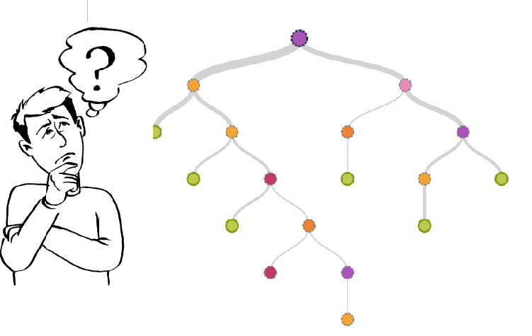
A decision tree is one of most frequently and widely used supervised machine learning algorithms that can perform both regression and classification tasks.
The intuition behind the decision tree algorithm is simple, yet also very powerful.
Everyday we need to make numerous decisions, many smalls and a few big.
So, Whenever you are in a dilemna, if you'll keenly observe your thinking process. You'll find that, you are unconsciously using decision tree approcah or you can also say that decision tree approach is based on our thinking process.

- A decision tree split the data into multiple sets.Then each of these sets is further split into subsets to arrive at a decision.
- It is a very natural decision making process asking a series of question in a nested if then else statement.
- On each node you ask a question to further split the data held by the node.
So, lets understand what is a decision tree with a help of a real life example.
Consider a scenario where a person asks you to lend them your car for a day, and you have to make a decision whether or not to lend them the car. There are several factors that help determine your decision, some of which have been listed below:
-
Is this person a close friend or just an acquaintance?
- If the person is just an acquaintance, then decline the request;
- if the person is friend, then move to next step.
-
Is the person asking for the car for the first time?
- If so, lend them the car,
- otherwise move to next step.
-
Was the car damaged last time they returned the car?
- If yes, decline the request;
- if no, lend them the car.
The decision tree for the aforementioned scenario looks like this:
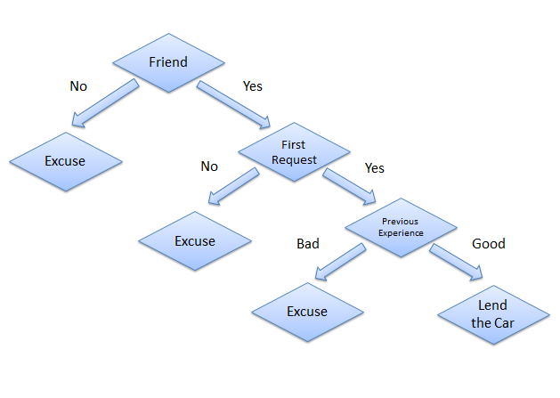
The structure of decision tree resembles an upside down tree, with its roots at the top and braches are at the bottom. The end of the branch that doesnt split any more is the decision or leaf.

Now, lets see what is Decision tree algorithm.
Decision tree is a type of supervised learning algorithm (having a pre-defined target variable) that is mostly used in classification problems.
- It works for both categorical and continuous input and output variables.
- In this technique, we split the population or sample into two or more homogeneous sets (or sub-populations) based on most significant splitter / differentiator in input variables.
Let’s look at the basic terminology used with Decision trees:
-
Root Node:
It represents entire population or sample and this further gets divided into two or more homogeneous sets. -
Splitting:
It is a process of dividing a node into two or more sub-nodes. -
Decision Node:
When a sub-node splits into further sub-nodes, then it is called decision node. -
Leaf/ Terminal Node:
Nodes do not split is called Leaf or Terminal node.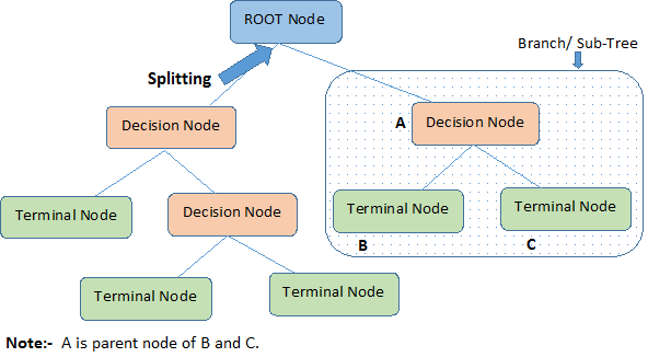
-
Pruning:
When we remove sub-nodes of a decision node, this process is called pruning. You can say opposite process of splitting. -
Branch / Sub-Tree:
A sub section of entire tree is called branch or sub-tree. -
Parent and Child Node:
A node, which is divided into sub-nodes is called parent node of sub-nodes where as sub-nodes are the child of parent node.
Types of decision tree is based on the type of target variable we have. It can be of two types:
-
Categorical Variable Decision Tree:
- Decision Tree which has categorical target variable then it called as categorical variable decision tree.
-
Continuous Variable Decision Tree:
- Decision Tree has continuous target variable then it is called as Continuous Variable Decision Tree.
- Decision Tree has continuous target variable then it is called as Continuous Variable Decision Tree.
Example:
- Let’s say we have a problem to predict whether a customer will pay his renewal premium with an insurance company (Yes/ No).
For this we are predicting values for categorical variable. So, the decision tree approach that will be used is Categorical Variable Decision Tree.
- Now, suppose insurance company does not have income details for all customers. But, we know that this is an important variable, then we can build a decision tree to predict customer income based on occupation, product and various other variables.
In this case, we are predicting values for continuous variable. So , This approach is called Continuous Variable Decision Tree.
Homogenous populations are alike and heterogeneous populations are unlike.
- A heterogenous population is one where individuals are not similar to one another.
- For example, you could have a heterogenous population in terms of humans that have migrated from different regions of the world and currently live together. That population would likely be heterogenous in regards to height, hair texture, disease immunity, and other traits because of the varied background and genetics.
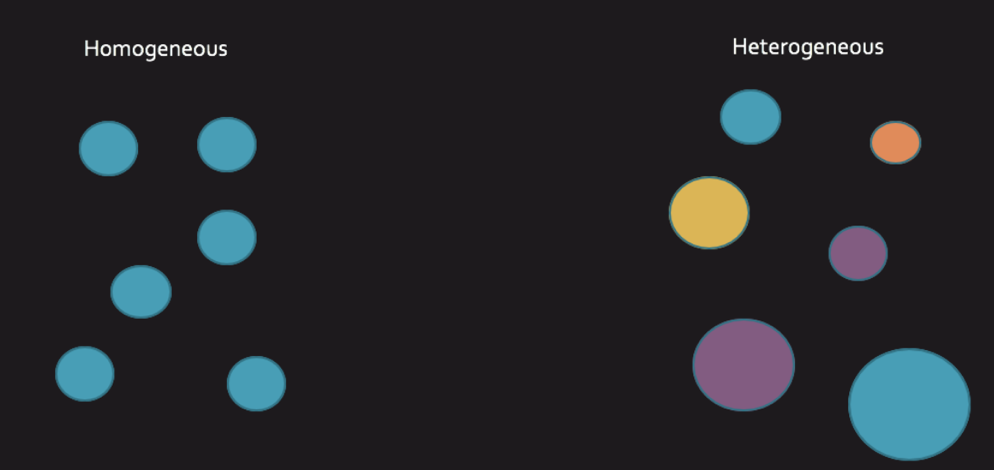
Note: In real world you would never get this level of homogeniety. So out of the hetrogenous options you need to select the one having maximum homoginiety. To select the feature which provide maximum homoginety we use gini & entropy techniques.
What Decision tree construction algorithm will try to do is to create a split in such a way that the homogeneity of different pieces must be as high as possible.
Example
Let’s say we have a sample of 30 students with three variables:
- Gender (Boy/ Girl)
- Class (IX/ X) and,
- Height (5 to 6 ft).
15 out of these 30 play cricket in leisure time. Now, I want to create a model to predict who will play cricket during leisure period? In this problem, we need to segregate students who play cricket in their leisure time based on highly significant input variable among all three.
This is where decision tree helps, it will segregate the students based on all values of three variables and identify the variable, which creates the best homogeneous sets of students (which are heterogeneous to each other). In the snapshot below, you can see that variable Gender is able to identify best homogeneous sets compared to the other two variables.

As mentioned above, decision tree identifies the most significant variable and it’s value that gives best homogeneous sets of population. Now the question which arises is, how does it identify the variable and the split? To do this, decision tree uses various algorithms, which we will shall discuss in the following section.
4.5 How does a tree decide where to split?
The decision of making strategic splits heavily affects a tree’s accuracy. The decision criteria is different for classification and regression trees.
Decision trees use multiple algorithms to decide to split a node in two or more sub-nodes. The creation of sub-nodes increases the homogeneity of resultant sub-nodes. In other words, we can say that purity of the node increases with respect to the target variable. Decision tree splits the nodes on all available variables and then selects the split which results in most homogeneous sub-nodes.
The algorithm selection is also based on type of target variables. Let’s look at the most commonly used algorithms in decision tree:
4.5.1 Gini Index
Gini index says, if we select two items from a population at random then they must be of same class and probability for this is 1 if population is pure.
- It works with categorical target variable “Success” or “Failure”.
- It performs only Binary splits
- Higher the value of Gini higher the homogeneity.
- CART (Classification and Regression Tree) uses Gini method to create binary splits.
Steps to Calculate Gini for a split
- Calculate Gini for sub-nodes, using formula sum of square of probability for success and failure (1
-p2-q2). - Calculate Gini for split using weighted Gini score of each node of that split
Example:
– Referring to example used above, where we want to segregate the students based on target variable ( playing cricket or not ). In the snapshot below, we split the population using two input variables Gender and Class. Now, I want to identify which split is producing more homogeneous sub-nodes using Gini index.
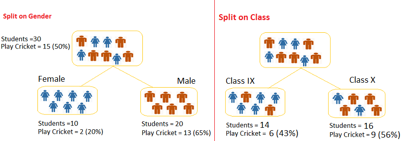
Gini for Root node:
- 1
-(0.5*0.5)-(0.5*0.5) = 0.50
Split on Gender:
- Gini for sub-node Female
- 1
-(0.2*0.2)-(0.8*0.8) = 0.32
- 1
- Gini for sub-node Male
- 1
-(0.65*0.65)-(0.35*0.35) = 0.45
- 1
- Weighted Gini for Split Gender
- (10/30)
*0.32+(20/30)*0.45 = 0.41
- (10/30)
Split on Class :
- Gini for sub-node Class IX =
- 1
-(0.43*0.43)-(0.57*0.57) = 0.49
- 1
- Gini for sub-node Class X =
- 1
-(0.56*0.56)-(0.44*0.44) = 0.49
- 1
- Calculate weighted Gini for Split Class
- (14/30)
*0.51+(16/30)*0.51 = 0.49
- (14/30)
Above, you can see that:
Gini score for Split on Gender < Gini score for Split on Class.
Also, Gini score for Gender < Gini score for root node.
Hence, the node split will take place on Gender.
4.5.2 Information Gain:
Look at the image below and think which node can be described easily.
I am sure, your answer is C because it requires less information as all values are similar. On the other hand, B requires more information to describe it and A requires the maximum information.
In other words, we can say that C is a Pure node, B is less Impure and A is more impure.
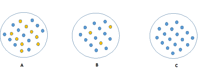
Now, we can build a conclusion that:
- less impure node requires less information to describe it.
- more impure node requires more information.
Information theory is a measure to define this degree of disorganization in a system by a parameter known as Entropy.
- If the sample is completely homogeneous, then the entropy is zero and
- If the sample is an equally divided (50% – 50%), it has entropy of one.
Entropy can be calculated using formula:
 where,
p & q is probability of success and failure respectively in that node.
-
Information Gain = 1 - Entropy.
- The model will choose the split which facilitates maximum information gain, which in turn means minimum Entropy.
- So, it chooses the split which has lowest entropy compared to parent node and other splits.
- The lesser the entropy, the better it is.
Steps to calculate entropy for a split:
- Calculate entropy of parent node
- Calculate entropy of each individual node of split and
- Calculate weighted average of all sub-nodes available in split.
- Caluclate the Information Gain in various split options w.r.t parent node
- Choose the split with highest Information Gain.
Example: Let’s use this method to identify best split for student example.
-
Entropy for parent node
-
-(15/30) log2 (15/30)–(15/30) log2 (15/30) = 1.
Here 1 shows that it is a impure node.
-
-
Entropy for Female node
-
-(2/10) log2 (2/10)–(8/10) log2 (8/10) = 0.72
-
-
Entropy for male node
-
-(13/20) log2 (13/20)–(7/20) log2 (7/20) = 0.93
-
-
Entropy for split Gender = Weighted entropy of sub
-nodes- (10/30)
*0.72 + (20/30)*0.93 = 0.86
- (10/30)
-
Information Gain for split Gender = Entropy of Parent Node
-Weighted entropy for Split Gender- 1
-0.86 = 0.14
- 1
-
Entropy for Class IX node,
-
-(6/14) log2 (6/14)–(8/14) log2 (8/14) = 0.99
-
-
Entropy for Class X node,
-
-(9/16) log2 (9/16)–(7/16) log2 (7/16) = 0.99.
-
-
Entropy for split Class,
- (14/30)
*0.99+(16/30)*0.99 = 0.99
- (14/30)
-
Information Gain for split Class = Entropy of Parent Node
-Weighted entropy for Split Class- 1
-0.99 = 0.01
- 1
Observe that:
Information Gain for Split on Gender > Information Gain for Split on Class,
So, the tree will split on Gender.
-
Easy to Understand:
- Decision tree output is very easy to understand even for people from non-analytical background. It does not require any statistical knowledge to read and interpret them.
- Its graphical representation is very intuitive and users can easily relate their hypothesis.
-
Less data cleaning required:
- It requires less data cleaning compared to some other modeling techniques.
- It is not influenced by outliers and missing values to a fair degree.
-
Data type is not a constraint:
- It can handle both numerical and categorical variables.
-
Non Parametric Method:
- Decision tree is considered to be a non-parametric method. This means that decision trees have no assumptions about the space distribution and the classifier structure.
4.7 Shortcomings of Decision Trees
-
Over fitting:
- Over fitting is one of the most practical difficulty for decision tree models. This problem gets solved by setting constraints on model parameters and pruning (discussed in detailed below).
-
Not a great contributor for regression:
- While working with continuous numerical variables, decision tree looses information when it categorizes variables in different categories.
X = titanic.loc[:,titanic.columns != 'Survived']
X.head()
y = titanic.Survived
from sklearn.model_selection import train_test_split
X_train, X_test, y_train, y_test = train_test_split(X, y, test_size=0.20, random_state=1)
print(X_train.shape)
print(y_train.shape)
To apply any machine learning algorithm on your dataset, basically there are 4 steps:
- Load the algorithm
- Instantiate and Fit the model to the training dataset
- Prediction on the test set
- Calculating the accuracy of the model
The code block given below shows how these steps are carried out:
from sklearn import tree
    model = tree.DecisionTreeClassifier(criterion='gini')
    model.fit(X, y)
    predicted= model.predict(x_test)
from sklearn import tree
model = tree.DecisionTreeClassifier(random_state = 0)
model.fit(X_train, y_train)
- Plotting our model of decision tree
import sys
!{sys.executable} -m pip install graphviz
!{sys.executable} -m pip install pydotplus
!{sys.executable} -m pip install Ipython
import pydotplus
from IPython.display import Image

dot_tree = tree.export_graphviz(model, out_file=None,filled=True, rounded=True,
                                special_characters=True, feature_names=X.columns)
graph = pydotplus.graph_from_dot_data(dot_tree)

Image(graph.create_png())
y_pred_train = model.predict(X_train)
y_pred_test = model.predict(X_test) # make predictions on the testing set
- Now lets see some model evaluation techniques.
Error is the deviation of the values predicted by the model with the true values.
We will use accuracy score and confusion matrix for evaluation.
from sklearn.metrics import accuracy_score
print('Accuracy score for test data is:', accuracy_score(y_test,y_pred_test))
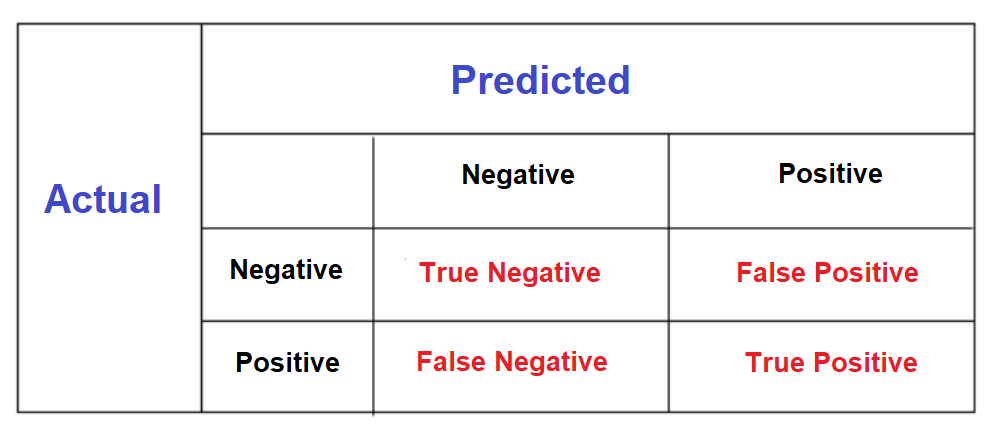
A confusion matrix is a summary of prediction results on a classification problem.
The number of correct and incorrect predictions are summarized with count values and broken down by each class.
Below is a diagram showing a general confusion matrix.
from sklearn.metrics import confusion_matrix

confusion_matrix = pd.DataFrame(confusion_matrix(y_test, y_pred_test))

confusion_matrix.index = ['Actual Died','Actual Survived']
confusion_matrix.columns = ['Predicted Died','Predicted Survived']
print(confusion_matrix)
This means 88 + 51 = 139 correct predictions & 22 + 18 = 40 false predictions.
6. Decision Tree with Gridsearch
Applying GridsearchCV method for exhaustive search over specified parameter values of estimator.
To know more about the different parameters in decision tree classifier, refer the documentation.
Below we will apply gridsearch over the following parameters:
- criterion
- max_depth
- max_features
You can change other parameters also and compare the impact of it via calculating accuracy score & confusion matrix
from sklearn.tree import DecisionTreeClassifier
from sklearn.model_selection import GridSearchCV

decision_tree_classifier = DecisionTreeClassifier(random_state = 0)


tree_para = [{'criterion':['gini','entropy'],'max_depth': range(2,60),
                             'max_features': ['sqrt', 'log2', None] }]


grid_search = GridSearchCV(decision_tree_classifier,tree_para, cv=10, refit='AUC')
grid_search.fit(X_train, y_train)
- Using the model for prediction
y_pred_test1 = grid_search.predict(X_test)
- Model Evaluation using accuracy_score
from sklearn.metrics import accuracy_score
print('Accuracy score for test data is:', accuracy_score(y_test,y_pred_test1))
- Model Evaluation using confusion matrix
from sklearn.metrics import confusion_matrix

confusion_matrix = pd.DataFrame(confusion_matrix(y_test, y_pred_test1))

confusion_matrix.index = ['Actual Died','Actual Survived']
confusion_matrix.columns = ['Predicted Died','Predicted Survived']
print(confusion_matrix)
You can see 95 + 49 = 144 correct predictions & 24 + 11 = 35 false predictions.
Observations:
- With gridsearch accuracy_score increased from 0.765 to 0.804 and the number of correct predictions increased from 139 to 144 and number of false predictions decreased from 40 to 35.
